Deep Latent Variable Models and Variational Inference
$\newcommand{\posterior}{ p(z|x;\theta)}$ $\newcommand{\prior}{ p(z)}$ $\newcommand{\likelihood}{ p(x|z;\theta)}$ $\newcommand{\marglike}{ p(x;\theta)}$ $\newcommand{\fulllike}{ p(x, z;\theta)}$ $\newcommand{\variational}{ q(z;\phi)}$ $\newcommand{\KL}[2]{ \text{KL}(#1 \parallel #2)}$ $\newcommand{\ELBO}{ \mathcal{L}(\theta, \phi; x)}$ $\newcommand{\expectation}[2]{ \mathbb{E}_{#1}[#2]}$ $\newcommand{\Normal}[2]{ \mathcal{N}(#1, #2)}$ $\newcommand{\Real}{ \mathbb{R}}$
Mathematical Notation
Click to expand
Probability Distributions:
- $\posterior$ - Posterior distribution of latent variables given observed data
- $\prior$ - Prior distribution of latent variables
- $\likelihood$ - Likelihood of observed data given latent variables
- $\marglike$ - Marginal likelihood (evidence)
- $\fulllike$ - Joint distribution of observed and latent variables
- $\variational$ - Variational approximation to the posterior
Key Terms:
- $\ELBO$ - Evidence Lower BOund
- $\KL{q}{p}$ - Kullback-Leibler divergence from q to p
Variables:
- $x$ - Observed data
- $z$ - Latent variables
- $\theta$ - Generative model parameters
- $\phi$ - Variational parameters
- $w$ - Global latent variable (GMVAE)
- $l$ - Local/cluster-specific latent variable (GMVAE)
I’m a sucker for deep learning with a probabilistic interpretation, because I’m always asking myself two questions when I fit models:
- Why should I expect anything to be linear?
- Given that the answer to (a) is probably "You shouldn't", then why not parameterise a distribution with a neural net?
In this post, I describe a class of deep learning models that approximate posterior distributions via variational Bayesian inference, use them to build a clustering model, and show how the architecture can yield meaningful clusterings.
Latent Variable Models
A latent variable model assumes that observed data $\mathrm{x} \in \Real^N$ has a likelihood that depends on a latent variable $z$ and some generative model parameters $\theta$, $p(\mathrm{x} \mid z ; \theta)$. $z$ itself has prior $p(z)$. We can make these models “deep” by implementing the probability $p(x \mid z; \theta)$ using a neural network. For instance, we may assume $z \sim \Normal{\mu}{I}$ for $z \in \Real^k, k < N$ and $p(x\mid z; \theta, W) = \mathrm{softmax}(Wh)$ where $h$ is the output of a neural network and $W$ is learnable. Latent models allow us to:
- Group documents by clustering their latent representations
- Generate new values of $x$ by sampling $z$. This, to me, feels like sampling the posterior predictive distribution. Although it is not strictly the same thing because we are not sampling from $\posterior$.
- If we trust the resulting distributions, the generated values of $x$ can be used for anomaly detection, causal inference, etc.
I’ve been interested in deep learning for parameterisation of probability distributions for a while, because I constantly encounter situations where I want to flexibly describe how certain distributional parameters vary as functions of some data, don’t want to commit to a functional form, and would like a posterior distribution to do inference. I’ve tried using Gaussian Processes for this, but there are issues of size because the covariance matrix scales quadratically with the number of data points and needs to be inverted.
The key sources for this blogpost are Kim, Wiseman and Rush’s A Tutorial on Deep Latent Variable Models of Natural Language and the Bishop(s) Deep Learning book
Variational Inference
In some cases, latent variable models can have tractable posteriors and we can find $\theta$ that maximises the marginal likelihood $\marglike$ via methods like Expectation Maximisation. Unfortunately, when we parameterise a latent variable model with a neural network, we lose the ability to write down the posterior and must resort to approximations. Variational inference is a method for approximating a posterior distribution with a distribution $\variational$ parameterised by $\phi$. Our objective is to maximise the log marginal likelihood $\marglike$. We do this by defining a lower bound on the marginal likelihood
\[\begin{align*} \marglike &= \int \variational \log \marglike \, dz \\ &= \int \variational \log \frac{\fulllike}{\posterior} \, dz \\ &= \int \variational \log \left[\frac{\fulllike}{\variational} \frac{\variational}{\posterior}\right] \, dz \\ &= \int \variational \log \left[\frac{\fulllike}{\variational}\right] \, dz + \int \variational \log \left[\frac{\variational}{\posterior}\right] \, dz \\ &= \expectation{\variational}{\left[\log \frac{\fulllike}{\variational}\right]} + \KL{\variational}{\posterior} \\ &:= \ELBO + \KL{\variational}{\posterior} \\ &\geq \ELBO \end{align*}\]In other words, we can decompose the marginal likelihood into two components: the KL divergence between the variational approximation and the posterior, and the term $\ELBO := \expectation{\variational}{\left[log\ \frac{\fulllike}{\variational}\right]}$, which is called the Evidence Lower Bound, or ELBO. It is a lower bound on the marginal likelihood because the KL term is always non-negative. Thus, optimising this bound allows us to optimise the likelihood.
Ideally, we have variational parameters $[\phi^{(i)}, …,\phi^{(N)}]$ for each of the $N$ data points in our dataset. Summing over the log likelihood for our data, the lower bound becomes $\sum_{i=1}^{N}\mathcal{L}(\theta, \phi^{(i)}; x^{(i)})$
Amortising The Variational Distribution
For a large dataset, having as many variational parameters as data points becomes unwieldy. Luckily we can avoid this by training a neural network to approximate the variational distribution. For instance, if we assume our variational distribution is Gaussian with a diagonal covariance, we can train a neural network to output the $\mu$ and $\sigma$ for each distribution. We achieve this by a decomposition of $\ELBO$
\[\ELBO = \expectation{\variational}{\ln\likelihood} - \KL{\variational}{\prior}\]Now our objective can be maximised by maximising the expectation of the log-likelihood over the variational distribution and minimising the (always non-negative) KL distance between the prior and the variational distribution. The expectation is estimated by sampling from $\variational$ and taking the mean of $\likelihood$. If we pick our variational family and our prior to be Gaussian and $\Normal{0}{1}$, respectively, the KL divergence can be calculated analytically.
Variational Autoencoders
The amortisation process combined with a neural network for generating the parameters of $\likelihood$ gives rise to an architecture known as a variational autoencoder. The first step in the model is to generate the parameters for the variational approximation to the posterior by passing x as input to an encoder network. Then $z$ is sampled from the posterior and passed as input to a decoder network, which generates parameters for a normal approximation to the likelihood.
These models have very exciting possibilities: you can generate data points by sampling the latent space, project your data onto a (hopefully meaningful) latent space, calculate posterior inference, etc.
Gaussian Mixture Variational Autoencoders
Here, I replicate the model architecture for the paper Deep Unsupervised Clustering with Gaussian Mixture Variational Autoencoders (henceforth the GMVAE paper). This paper interested me because clustering via mixture models can be very useful, but sampling a cluster assignment in a neural net results in a discontinuity that breaks differentiation. I’ll briefly describe the model components here (using slightly different notation than the paper): \(\begin{align} w &\sim \mathcal{N}(0, I) \tag{1a} \\ z &\sim \text{Mult}(\pi) \tag{1b} \\ l|z, w &\sim \prod_{k=1}^{K} \mathcal{N}\left(\mu_{z_k}(w; \beta), \text{diag}\left(\sigma^2_{z_k}(w; \beta)\right)\right)^{z_k} \tag{1c} \\ x|l &\sim \mathcal{N}\left(\mu(l; \theta), \text{diag}\left(\sigma^2(l; \theta)\right)\right) \text{ or } \mathcal{B}\left(\mu(l; \theta)\right) \tag{1d} \end{align}\)
In English, there are three latent variables:
- $z$, a one-hot encoded vector where the nonzero element is the cluster assignment, with prior $\text{Mult}(\pi)$
- $w$, which determines the means and variances of the various clusters via the networks $\mu_{z_k}(w; \beta)$ and $\sigma^2_{z_k}(w; \beta)$. $w$ has prior $\mathcal{N}(0, I)$
- $l$, which determines the likelihood via the networks $\mu(l; \theta)$ and $\sigma^2(x; \theta)$
Interestingly, they calculate a posterior for $z$ and reconstruct the ELBO in such a way that the model need not sample the discrete variable $z$ in the forward pass, retaining differentiability. Note that sampling a normal distribution for the likelihood and variational distributions is differentiable because we can generate $\mu$ and $\sigma$, then sample $n$ from $\Normal{0}{1}$ and do the old-fashioned $x = \mu + n\sigma$, which results in $x \sim \Normal{\mu}{\sigma^2}$. This maintains differentiability because the sampled $x$ is a differentiable function of the network outputs $\mu$ and $\sigma$.
What the GMVAE paper amounts to is a variational autoencoder consisting of an encoder for $w$ and $l$, a network for the conditional prior of $l$, a decoder network that maps $l \to x$, and a slightly more complicated loss function than the standard ELBO decomposition. The details are in the paper.
A PyTorch implementation of the model is below:
GMVAE Class Implementation
Click to view
import torch
from torch import nn
import torch.nn.functional as F
from torch.distributions import Normal, Categorical
from collections import OrderedDict
from typing import Tuple, Callable, Optional, List
def layer_from_list(dims:list[int], name:str, norm = True, negative = True, act:Callable=nn.Tanh) -> nn.Module:
    """
    Create a sequential list of layers
    """
    layers = OrderedDict()
    for i in range(1,len(dims)):
        layers[f'{name}_{i}'] = nn.Linear(dims[i-1], dims[i])
        if not (negative and i == len(dims)-1): #Skip last decoder activation to get negative reconstructions
            layers[f"{name}_activ_{i}"] = act()
        if norm and i < len(dims)-1:
            layers[f"{name}_norm_{i}"] = nn.LayerNorm(dims[i])
    return nn.Sequential(layers)


class GMVAE(nn.Module):
    def __init__(
        self,
        input_dim: int,
        w_dim: int,
        l_dim: int,
        enc_dim: List[int],
        dec_dim: List[int],
        k: int = 2,
        xav: bool = False
    ) -> None:
        """
        Gaussian Mixture Variational Autoencoder (GMVAE) implementation.

        This model learns a hierarchical latent representation with three latent variables:
        - w: A continuous latent variable that captures global structure
        - l: A continuous latent variable that captures local/cluster-specific structure
        - z: A discrete latent variable for cluster assignment (categorical)

        The generative model follows: p(x|l) * p(l|w,z) * p(w) * p(z)
        where p(l|w,z) is a mixture of Gaussians conditioned on w and cluster z.

        Args:
            input_dim (int): Dimensionality of input data
            w_dim (int): Dimensionality of global latent variable w
            l_dim (int): Dimensionality of local latent variable l
            enc_dim (list[int]): Hidden layer dimensions for encoder network
            dec_dim (list[int]): Hidden layer dimensions for decoder network
            k (int, optional): Number of mixture components/clusters. Defaults to 2.
            xav (bool, optional): Whether to use Xavier initialization. Defaults to False.

        Architecture:
            - Encoder: maps x -> (w_mu, w_sigma, l_mu, l_sigma)
            - Decoder: maps l -> (x_mu, x_sigma)
            - Prior network: maps w -> cluster-specific parameters for p(l|w,z)
        """

        """
        GMVAE

        note that instead of x for the latent dim, I use x for the input and l for the latent dimension
        """
        super().__init__()
        self.input_dim = input_dim
        self.k = k
        self.w_dim = w_dim
        self.l_dim = l_dim
        self.cat_dist = Categorical(probs=torch.FloatTensor([1 / k] * k))

        self.decoder = layer_from_list([l_dim] + dec_dim + [input_dim * 2], "decoder")
        # Varational networks. First 2*w_dim outputs are mu and ln_sigmas for the w, the remainder are the l dim
        enc_dim = [input_dim] + enc_dim + [w_dim * 2 + l_dim * 2]
        self.encoder = layer_from_list(enc_dim, "encoder", norm=False, act = nn.ReLU)
        # p(l|w,z) network for conditional prior and z posterior inference
        # input is w_dim dim
        # The outputs are 2k * l_dim which are chunked in to k tensors
        # The first l_dim in each chunk are the means for that cluster, the remainder are log variances
        self.p_l_network = layer_from_list([w_dim, 120, l_dim * 2 * self.k], "p(x|w,z)", act=nn.Tanh, norm=False)

        if xav:
            for m in self.modules():
                if isinstance(m, nn.Linear):
                    # Xavier/Glorot initialization for linear layers
                    nn.init.xavier_uniform_(m.weight)
                    if m.bias is not None:
                        nn.init.constant_(m.bias, 0)

    def reparameterise(
        self,
        mu: torch.Tensor,
        ln_sigma: torch.Tensor,
    ) -> torch.Tensor:
        eps = torch.randn_like(mu)

        l = mu + ln_sigma.exp() * eps
        return l

    def cluster_params(self, params: torch.Tensor, z: torch.Tensor) -> Tuple[torch.Tensor, torch.Tensor]:
        """
        Get the appropriate cluster parameters given the cluster assignments z
        """

        clusters = torch.chunk(params, self.k, -1)
        # z is (batch_size,), mus and ln_sigmas are tuples of (batch_size, latent_dim)
        # Stack mus and ln_sigmas to shape (k, batch_size, latent_dim)
        clusters_stacked = torch.stack(clusters, dim=0)
        selected_clusters = clusters_stacked[z, torch.arange(z.size(0))]
        mu, ln_sigma = torch.chunk(selected_clusters, 2, dim=-1)

        return mu, ln_sigma

    def sample(self, N: int = 1000, z: Optional[List[int]] = None, w: Optional[List[float]] = None) -> torch.Tensor:
        device = next(self.parameters()).device
        if w is None:
            w = torch.distributions.MultivariateNormal(torch.zeros((self.w_dim)), torch.eye(self.w_dim)).sample((N,)).to(device)
        if z is None:
            z = torch.distributions.Categorical([1/self.k] * self.k).sample(N).to(device)

        cp = self.p_l_network(w)
        l_mu, l_sigma = self.cluster_params(cp, z)

        l = self.reparameterise(l_mu, l_sigma)

        y_mu, y_ln_sigma = torch.chunk(self.decoder(l),2, dim = -1)

        y = self.reparameterise(y_mu, y_ln_sigma)
        return y


    def forward(self, x: torch.FloatTensor, cluster_params: bool = True) -> Tuple[torch.Tensor, torch.Tensor, Optional[torch.Tensor], torch.Tensor, torch.Tensor, torch.Tensor, torch.Tensor, torch.Tensor]:
        device = x.device
        h = self.encoder(x)
        w_params, l_params = torch.split(h, [self.w_dim * 2, self.l_dim * 2], dim=-1)
        w_mu, w_ln_sigma = torch.chunk(w_params, 2, dim=-1)
        l_mu, l_ln_sigma = torch.chunk(l_params, 2, dim=-1)

        w = self.reparameterise(w_mu, w_ln_sigma)
        l = self.reparameterise(l_mu, l_ln_sigma)

        cp = None
        if cluster_params:
            cp = self.p_l_network(w)

        recon_mu, recon_ln_sigma = torch.chunk(self.decoder(l), 2, dim=-1)

        return recon_mu, recon_ln_sigma, cp, w_mu, w_ln_sigma, l_mu, l_ln_sigma, l

    def conditional_prior(self, w_mu: torch.Tensor, w_ln_sigma: torch.Tensor, l_mu: torch.Tensor, l_ln_sigma: torch.Tensor, L: int = 5) -> torch.Tensor:
        result = 0
        for _ in range(L):
            w_j = self.reparameterise(w_mu, w_ln_sigma)
            l_j = self.reparameterise(l_mu, l_ln_sigma)
            cp = self.p_l_network(w_j)
            clusters = torch.chunk(cp, self.k, dim = -1)
            z_posterior = torch.chunk(self.cluster_posterior(cp, l_j), self.k, 0)
            for k in range(self.k):
                cluster_param = clusters[k]
                z_posterior_k = z_posterior[k]
                mu, ln_sigma = torch.chunk(cluster_param, 2, dim = -1)
                q_var = (2 * l_ln_sigma).exp()  # q variance
                p_var = (2 * ln_sigma).exp()
                KL = (0.5 *(q_var/p_var + 2*ln_sigma - 2*l_ln_sigma - 1 + (l_mu - mu).pow(2)/p_var)).sum(dim = -1)
                result += z_posterior_k*KL
        return (result/L).mean()

    def cluster_posterior(
        self,
        cp_params: torch.FloatTensor,
        latent: torch.Tensor,
    ) -> torch.FloatTensor:
        # split into k chunks
        clusters = torch.chunk(cp_params, self.k, -1)

        # joint distributions
        log_joint = [-1] * self.k
        for k in range(self.k):
            # select params for k_th cluster
            mu, ln_sigma = torch.chunk(clusters[k], 2, dim=-1)
            # p(z_k = 1, x)
            log_joint[k] = (
                torch.distributions.Independent(
                    torch.distributions.Normal(mu, ln_sigma.exp()), 1
                )
                .log_prob(latent)
            ) + torch.log(torch.tensor(1.0 / self.k, device=latent.device))
        # Stack on new dim corresponding to the joint probabilit for nonzero assignment for that cluster p(z_k =1 , x)
        log_joint = torch.stack(log_joint, dim=0)

        # Sum over z_k dim to get marginal p(x) for latent
        log_marginal = torch.logsumexp(log_joint, dim = 0)


        # P(z|x)
        return (log_joint - log_marginal).exp()

    def loss(
        self,
        x: torch.Tensor,
        w_mu: torch.Tensor,
        w_ln_sigma: torch.Tensor,
        l_mu: torch.Tensor,
        l_ln_sigma: torch.Tensor,
        cp: torch.Tensor,
        l: torch.Tensor,
        L: int = 30,
        lbd: float = 0
    ) -> Tuple[torch.Tensor, torch.Tensor, torch.Tensor, torch.Tensor, torch.Tensor, torch.Tensor]:
        z_posterior = self.cluster_posterior(cp, l)

        # q(l|x) samples
        variational_x = []
        for _ in range(L):
            l_sample = self.reparameterise(l_mu, l_ln_sigma)
            mc_recon_mu, mc_recon_ln_sigma = torch.chunk(self.decoder(l_sample), 2, dim=-1)
            log_prob = torch.distributions.Independent(
                torch.distributions.Normal(mc_recon_mu, mc_recon_ln_sigma.exp()), 1
            ).log_prob(x)
            variational_x.append(log_prob)
        recon_loss = torch.stack(variational_x, dim=0).mean(dim=0).mean()

        conditional_loss = self.conditional_prior(w_mu, w_ln_sigma, l_mu, l_ln_sigma)
        w_loss = torch.mean(-0.5 * torch.sum(1 + 2*w_ln_sigma - w_mu.pow(2) - (2*w_ln_sigma).exp(), dim=-1))
        # discrete KL divergence
        uniform_prior = torch.log(torch.tensor(1.0 / self.k, device=x.device))
        z_kl = 0
        for k in range(self.k):
            q_z_k = z_posterior[k] + 1e-10
            z_kl += q_z_k * (torch.log(q_z_k) - uniform_prior)

        z_loss = torch.clamp(z_kl.mean(), min=lbd)
        return -1 * recon_loss + conditional_loss + w_loss + z_loss, recon_loss, conditional_loss, w_loss, z_loss, z_kl.mean()
Reproducing The Spiral Data Experiment
The GMVAE paper describes a clustering experiment where the data consists of points in 2D space sampled from the arcs of 5 circles. Their data is on GitHub, so to test my implementation above, I attempted to replicate their architecture (given in their appendix A) and the results of their experiment. I used the same Adam setup as they did and clamped the $z$-prior term at 1.5 (their figure 3b). Training with my implementation is slightly brittle. Sometimes the $z$ prior term goes to zero even with clamping and the resulting clusters are heavily overlapping (i.e., the model exhibits what is known as “posterior collapse” and uses the prior cluster probabilities of $\frac{1}{k}$).
Still, when this doesn’t occur, the resulting clusters are meaningful. The top plot below shows KDE contours generated by setting the cluster to a particular value, sampling from the latent space associated with that cluster and decoding those samples. The points in the bottom plot have colours that correspond to $\underset{z}{\mathrm{argmax}}\ p(z\mid l,w,x)$, the most probable cluster for each data point according to the z-posterior.
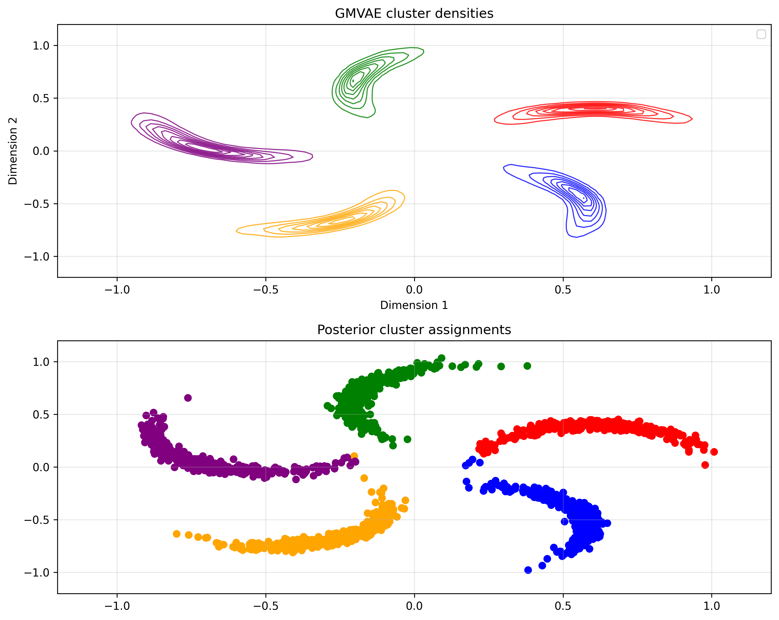
GMVAE is able to cluster points in this space meaningfully and the results demonstrate that the model has learned to associate different regions of the latent space with different clusters in the original data space.
Summary
Deep latent variable models offer a compelling framework for probabilistic machine learning that goes beyond the limitations of linear models and fixed distributional assumptions. By parameterising probability distributions with neural networks, we can capture complex, non-linear relationships in data while maintaining a principled Bayesian interpretation.
The GMVAE architecture showcases how we can extend standard variational autoencoders to handle discrete latent variables for clustering tasks. Despite some training brittleness (a common theme with these models), the approach successfully learns meaningful cluster assignments without requiring discrete sampling in the forward pass, preserving differentiability throughout.